Time-dependent strategy dynamics in a perceptual decision-making task
Abstract
Human perceptual estimation balances internal expectations with incoming sensory evidence. Although static switching models suggest that observers alternate between prior-dependent and evidence-tracking response modes, it remains unclear whether these switches are trial-independent or governed by dynamic, history-dependent cognitive states. The input-driven Hidden Markov Model (HMM) achieved lower held-out predictive negative log-likelihood than the static models on average, revealing that participants’ strategy use contains temporally structured dependencies. Furthermore, fitted transition parameters further indicated that state transition probabilities varied by trial-by-trial motion coherence and the angular distance between stimulus and the prior mean, although these covariate effects vary across subjects.
Introduction
This project used the Neuromatch Academy perceptual dot-motion decision-making datasetLaquitaine & Gardner, 2018. In this task, participants estimated the motion direction of random dots while two task variables were manipulated: 1) motion coherence (percentage of dots moving in the same direction), and 2) prior standard deviation (the sharpness of the presented dot distribution). A Bayesian observer integrates the noisy sensory measurement with the prior to form a single posterior estimate. In contrast, a switching observer selects between response modes, relying either on the prior mean or on the sensory evidence depending on their relative reliability. For example, when motion coherence is low, subjects tend to choose estimates from the prior distribution, leading to a bias toward estimates near the prior, whereas an increase in prior standard deviation introduces greater variability in subjects’ estimates. Previous results have shown that the switching observer model yielded a better fit than the Bayesian observer model, as it could account for the bimodality distribution of individuals’ estimates when the presented motion was very different from the constant prior experimental mean of 225˚.
We aimed to test whether switching behaviour is time-dependent and whether task variables such as motion coherence influence participants’ latent decision states. Recent reviews have challenged the assumption that decision strategies are stable across trials and have shown that models that deploy non-stationary dynamics, such as discrete-state switches, provide greater explanatory power for human behaviour than some standard static models Gunawan et al., 2022Urai, 2026. We therefore compared three models: Probabilistic Mixture model (PM), Weighted Mean model (WM) and an input-driven Hidden Markov Model.
Weighted Mean model with a global variance (WM)
Unlike a discrete-switching framework, this model assumes that on every trial t, the brain combines the prior and sensory evidence into a single integrated estimate. The relative contribution of sensory evidence versus prior is determined by a logistic function of task covariates and
i.e. the weight of selecting the evidence component on any given trial, , is determined by coherence and , the sensitivity to sensory clarity/ contrast, together with , the absolute magnitude of the displayed angle location relative to the prior.
The likelihood was modelled as a single von Mises distribution centred on the circular weighted mean () of the prior and evidence direction angle , with a single shared concentration parameter . The von Mises distribution is the circular analogue of the Gaussian distribution.
Probabilistic Mixture model (PM)
The original switching observer account suggests that participants do not always integrate prior and sensory evidence into a single response. Instead, responses may be generated from one of two distributions: a prior-centred distribution or an evidence-centred distribution. PM has the same model structure as WM, except that it assumes that the subject responds based on either the prior-centred distribution with concentration or the evidence-centred distribution with concentration . Here, the trial-wise evidence weight determines the probability that a response is generated from the evidence component rather than the prior component. We set the bounds of bcoh to be highly positive (10, 50), as we assume higher coherence drives the model to weight the physical evidence over the prior.
Evidence Likelihood:
Prior Likelihood:
On any single trial, the overall probability density of observing response is a weighted linear combination of the two components.
In full-data fits, PM had lower AIC and BIC than WM by 21,417.9 and 21,306.0 ponts, respectively. More importantly, blocked leave-one-run-out cross-validation showed that PM reduced held-out NLL relative to WM by a mean of 0.1028 per trial, (11)=4.57, p=0.0008. This indicates that participants’ responses were better described by discrete probabilistic switching than by continuous weighted averaging.
Input-driven Hidden Markov Model
Despite that PM model allows responses to switch between prior-centred and evidence-centred components, it treats each trial as independent. In other words, the probability of relying on evidence on trial is not directly influenced by the participant’s latent state on trial . A Hidden Markov model enables the capture of internal mental states, such as mind-wandering, by inferring a posterior probability over latent states for each trial Ashwood et al., 2022. In our model, the two hidden states correspond to prior and evidence modes, which represent distinct decision-making strategies, and were parametrised by a set of GLM weights that describe how subjects weigh different task covariates to make a decision in each state. The model was fitted using the Expectation Maximization (EM) algorithm with a maximum of 50 iterations and 5 random initializations. The solution with highest converged log-likelihood was retained.
Latent State Transitions
The transition is modelled using multinomial logistic regression. The discrete hidden states at time t are denoted as , which represents the discrete latent state at trial t, where = 0 corresponds to the Prior state and = 1 represents the Evidence state.
Given previous state the probability of transitioning to state depends on the trial-wise input vector , and which includes the current displayed angle and three levels of motion coherence. Prior standard deviation was not included as a transition input because it was not directly visible to participants on a trial-by-trial basis. The probability of jumping from the current state to the next state is a softmax over all possible next states. Here, represents the baseline, unnormalized transition bias independent of external task inputs. The vector represents the transition weights that depend on the destination state . These weights determine how strongly motion coherence and stimulus orientation modulate and shift behavioral strategies.
Emission Likelihoods
The emission model links each latent state to a response distribution. The likelihood of observed response is obtained by marginalising over the latent states:
Where the conditional state emissions are defined as:
State 0 (Prior state) captures responses clustered around the prior mean, whereas State 1 (Evidence state) captures responses clustered around the displayed stimulus direction.
Leave-one-block-out cross validated predictive negative log likelihood of the first four blocks (each block contains around 200 trials) was compared across the three models. The HMM had lower held-out NLL than PM on average and for 10 of 12 participants (Mean difference per trial = 0.0677, (11)=3.672, < 0.001), although the size and direction of the difference varied across individuals. Self-transition probabilities were generally high, indicating persistent latent-state assignments, although the degree of persistence varied substantially across participants (Figure 1). This result suggests that strategy switching is not only discrete, as captured by the PM model, but also temporally structured (Figure 2, Figure 3). Subject level examples further illustrate this temporal structure. Our study extends the switching observer phenomenon by providing a temporal account for individual differences in strategy switching (Figure 4). We compared subjects who showed improved HMM model-fitting scores, with highest and lowest error among the first 4 blocks. Importantly, both subjects may look switch-like, but subject 10 has a more persistent pattern with higher task error than subject 3, which hints at a non-optimal evidence use.
In conclusion, this study demonstrated that human observers may not lie on a one-dimensional Bayesian-vs-switching axis. Some subjects show more adaptive patterns of arbitration between the two states along with the increase of motion coherence, whereas others show blockwise strategy states. Evidence-state persistence was not significantly correlated with mean absolute error across subjects, =0.36, =0.25, =12. Future studies could explore more on the relationship of state transitions with subjects’ behavior and disentangle the psychological meaning behind an ‘evidence state’: whether it involves a strategic exploration or merely task engagement.
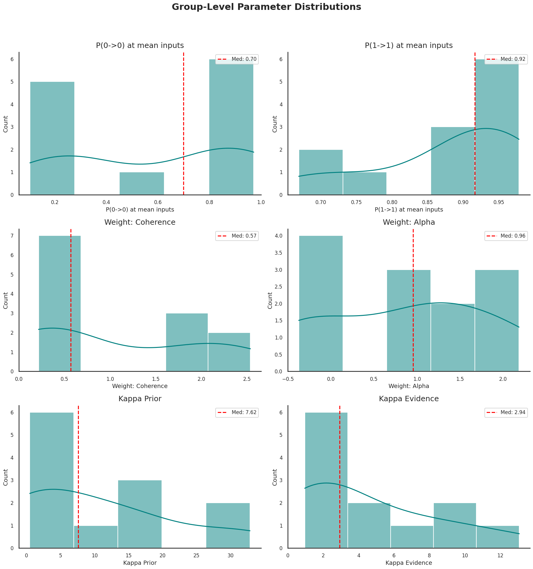
Figure 1:Group-level parameter distributions from the input-driven HMM model across subjects, N=12. P(0->1) and P(1->1) at mean inputs represent the transition probabilities into the evidence state when the input variables are zero. P(0->1) reflects switching from the prior state to the evidence state, whereas P(1->1) reflects persistence in the evidence state. Input weights for coherence and alpha describe how these covariates modulate the probability of transitioning into the evidence state. Positive weights indicate that higher values of the covariate increase the tendency to enter or remain in the evidence state. The alpha weight has a higher median value than the coherence weight, suggesting that the displayed angle has a stronger association with transitioning into the evidence state than coherence. Kappa_prior and kappa_evidence are concentration parameters of the von Mises emission distributions. Higher median compared with suggested that prior state responses are more precise around the prior mean than responses assigned to the evidence state were around the stimulus angle; Red dashed lines indicate group medians.
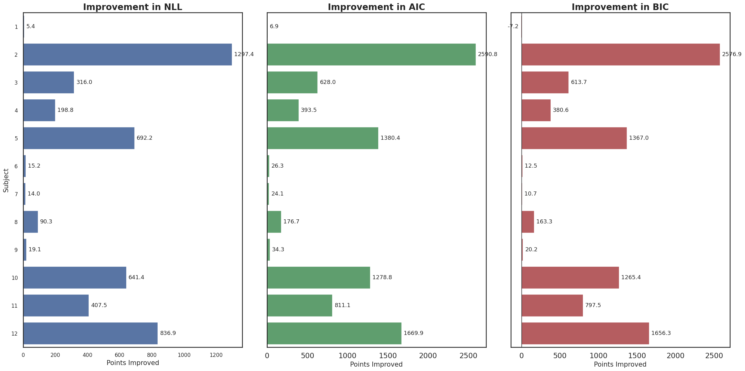
Figure 2:While a majority of subjects showed an improvement in model fitting scores, Subjects 1, 6, 7, 9 demonstrated near-zero, negligible shifts, with subject 1 showing a negative improvement score of -7.2.
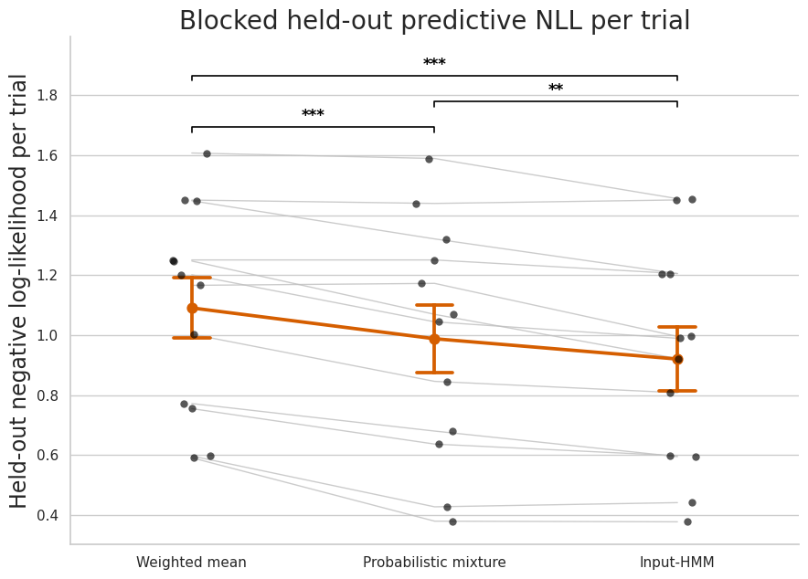
Figure 3:Block held out predictive negative log likelihood. Paired t-test results are shown. p < 0.001 ***, p < 0.01 **, p < 0.05 *
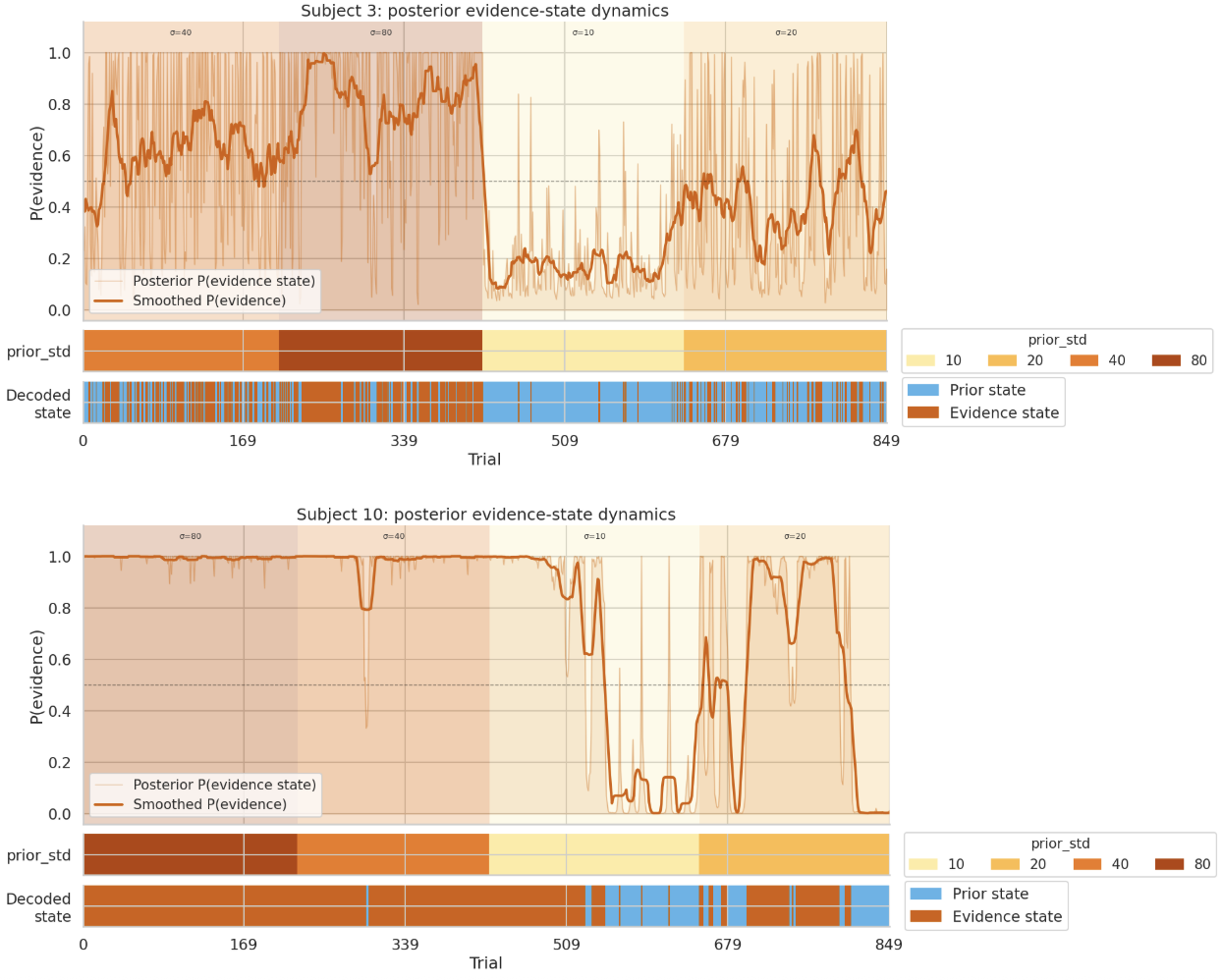
Figure 4:The plots show modelled input HMM latent-state probabilities of Subject 3 and 10, who had the lowest and the highest task error across the first four blocks. The orange curve indicates the probability of staying at the evidence state P(evidence). Higher prior standard deviation reflects higher task difficulty.
Acknowledgments
This work was supported by the Impact Scholars Program. We acknowledge the contributions of team members Shiva Kamkar, Shima Javadi, Mohammad Basiri.
Data Availability
Published via Impact Scholars; original development repository.
- Laquitaine, S., & Gardner, J. L. (2018). A Switching Observer for Human Perceptual Estimation. Neuron, 97(2), 462-474.e6. 10.1016/j.neuron.2017.12.011
- Gunawan, D., Hawkins, G. E., Kohn, R., Tran, M.-N., & Brown, S. D. (2022). Time-Evolving Psychological Processes over Repeated Decisions. Psychological Review, 129(3), 438–456. 10.1037/rev0000351
- Urai, A. E. (2026). Structure Uncovered: Understanding Temporal Variability in Perceptual Decision-Making. Trends in Cognitive Sciences, 30(1), 54–65. 10.1016/j.tics.2025.06.003
- Ashwood, Z. C., Roy, N. A., Stone, I. R., Urai, A. E., Churchland, A. K., Pouget, A., & Pillow, J. W. (2022). Mice Alternate between Discrete Strategies during Perceptual Decision-Making. Nature Neuroscience, 25(2), 201–212. 10.1038/s41593-021-01007-z