Low Built-Up Density Emerges as a Key Driver of Heat Extremes over the Sahel
Abstract
Urban heat islands threaten fast-growing Sahelian cities, yet causal drivers of surface heating remain unknown. Here we combine machine-learning classification (XGBoost, Random Forest, SVM) with spatial causal inference to disentangle correlation from causation among hotspot drivers in Ouagadougou, Burkina Faso. XGBoost generalised best (F1 = 0.70, κ = 0.67) while SHAP analysis identified built-up density as the dominant predictor. Geographical convergent cross-mapping confirmed it as a unidirectional cause of surface temperature, while spectral indices showed only bidirectional coupling despite strong correlations. Opposite to humid tropical cities, lower built-up density increases hotspot risk due to exposed bare soil. These findings point to compact urban form as a heat mitigation strategy.
Introduction
Urban heat islands (UHIs), in which cities are substantially warmer than surrounding rural areas, pose a growing public health threat, particularly in rapidly urbanizing regions of the Global South Tuholske et al., 2021. In sub-Saharan Africa, where urbanization rates are among the highest globally, the thermal consequences of land cover change are poorly understood due to limited ground-based monitoring infrastructure Seto et al., 2012. Ouagadougou, the capital of Burkina Faso, exemplifies this challenge: a Sahelian city experiencing rapid peri-urban expansion in a semi-arid climate where baseline temperatures already reach extreme levels during the March-May hot season.
Land surface temperature (LST), derivable from satellite thermal imagery, provides a spatially continuous proxy for surface energy balance and has been widely used to delineate thermal hotspots across urban environments Voogt & Oke, 2003. However, translating LST patterns into actionable planning insights requires moving beyond prediction to causal understanding and identifying which landscape features are genuine drivers of surface heating rather than mere correlates. Machine learning (ML) models can achieve high predictive accuracy but offer limited causal interpretability without complementary analytical frameworks.
This study maps thermal hotspots in Ouagadougou during the 2022-2024 hot season using Landsat-derived LST composites. We train and compare three ML classifiers XGBoost, Random Forest, and Support Vector Machine, on predictors spanning spectral indices, land cover density, topography, and proximity to water bodies and road networks Pekel et al., 2016. To move beyond correlation, we apply SHapley Additive exPlanations (SHAP) for predictor importance and Geographical Convergent Cross Mapping (GCCM; Gao et al., 2023) to infer causal directionality between variables. This combined predictive-causal approach replicates and extends the methodology of Hoang et al., 2025, originally applied to Da Nang, Vietnam, to test whether urban heat mechanisms identified in a humid tropical city transfer to a semi-arid Sahelian context with direct implications for climate-sensitive urban planning in West Africa Oke et al., 2017.
Methods
Data and processing
Land surface temperature (LST) was derived from Landsat 8 and 9 Collection 2 Level-2 Surface Temperature products, composited across the March-May hot season from 2022 to 2024. Scenes exceeding 20% cloud cover were excluded, per-pixel cloud and shadow masking was applied, and physically implausible values outside 20-60°C were rejected; a pixel-wise median composite was computed at 30m resolution.
We define intra-urban surface heat hotspots — distinct from the classical urban heat island (UHI) concept, which compares urban to surrounding rural temperatures — as pixels exceeding the study-area mean by more than one standard deviation (LST > μ + 1σ, Weng et al., 2004), yielding a binary classification of hotspot (1) versus non-hotspot (0). This relative threshold captures locally anomalous heating within the city rather than the city-versus-rural contrast that defines UHI. Of the 613,847 valid pixels covering the Ouagadougou administrative boundary, approximately 10.3% were classified as intra-urban heat hotspots (hereafter “hotspots”).
Eight predictor variables were compiled from spectrally and temporally independent datasets to avoid analytical circularity with the Landsat-derived target (Table 1). All layers were resampled to a common 30m UTM Zone 30N grid in a final step.
Data sources and processing.
| Feature | Description | Source | Period | Processing |
|---|---|---|---|---|
| Land Surface Temperature (LST) | Surface temperature | Landsat 8/9 Collection 2, Level 2 | Mar–May 2022–2024 | Cloud-masked median composite; ST_B10 × 0.00341802 + 149.0 − 273.15 |
| NDVI | Spectral proxy for vegetation presence | Sentinel-2 L2A | Mar–May 2024 | NDVI = (B8 - B4) / (B8 + B4) |
| NDBI | Spectral proxy for urban build-up | Sentinel-2 L2A | Mar–May 2024 | NDBI = (B11 - B8) / (B11 + B8) |
| BSI | Spectral proxy for exposed soil | Sentinel-2 L2A | Mar–May 2024 | BSI = ((B11 + B4) - (B8 + B2)) / ((B11 + B4) + (B8 + B2)) |
| DEM | Elevation | Copernicus GLO-30 DEM | Static | Mosaic of tiles |
| Distance to water | Distance in meters to water bodies | JRC Global Surface Water v1.4 | Static | Euclidean distance; ≥70% occurrence threshold Pekel et al., 2016 |
| Distance to roads | Distance in meters to roads | OpenStreetMap via BBBike.org | Static | Euclidean distance |
| Built-up density | Local urban surface fraction | ESA WorldCover v200 | 2021 | Fraction within a 90 m radius neighborhood |
| Green space density | Local vegetation cover fraction | ESA WorldCover v200 | 2021 | Fraction within a 90 m radius neighborhood |
Modelling and feature importance
Three binary classifiers were trained on all predictors to classify hotspot occurrence using the full set of 613,847 valid pixels: XGBoost Chen & Guestrin, 2016, Random Forest Breiman, 2001, and a Support Vector Machine (SVM) with RBF kernel. Data were randomly split 70/30 train/test following Hoang et al., 2025.
Hyperparameters were selected via five-fold cross-validated grid search (GridSearchCV, scoring = accuracy, n_jobs = -1). Models were evaluated on both training and test sets using accuracy, precision, recall, F1 score, and Cohen’s Kappa. The model with the highest generalization performance was selected for spatial prediction and interpretability analysis.
To rank which predictors contribute most to the model’s hotspot classifications, feature importance was quantified using SHapley Additive exPlanations (SHAP; Lundberg & Lee, 2017) via TreeExplainer on the held-out test set. SHAP values decompose each prediction additively across features in a game-theoretic framework, providing both global importance rankings (mean |SHAP value|) and directional insights into how each predictor relates to model-estimated hotspot probability. SHAP quantifies predictive contribution, not causation; the causal inference in the next section addresses directionality.
Causal inference
To test whether SHAP-identified predictors causally influence LST or merely co-vary with it, we applied Geographical Convergent Cross Mapping (GCCM; Gao et al., 2023) as implemented in the spEDM R package Lv, 2025. GCCM extends Sugihara et al., 2012 convergent cross mapping (CCM) to spatial cross-sectional data and tests whether one variable’s state space can predict another’s.
For each predictor–LST pair, bidirectional GCCM was run on the 150m aggregated raster with embedding dimension E = 3 and spatial lag τ = 1 (150m), using 2,000 randomly sampled prediction points. Causal direction was determined by three criteria following Gao et al., 2023: (1) convergence (Kendall’s τ > 0 for cross-map skill ρ vs. library size), (2) significance at the largest library size (p < 0.05), and (3) non-overlapping 95% Fisher-z confidence intervals between forward and reverse directions.
Results
Descriptive Statistics
During the March-May hot season, LST across Ouagadougou averaged 46.0 °C (SD = 2.1 °C, range 31.0-52.5 °C), with 10.3% of pixels exceeding the hotspot threshold (LST > 48.1 °C). The landscape is semi-arid with low vegetation (median NDVI = 0.11) and minimal topographic relief (274-347m). Built-up density is bimodal, reflecting a dense urban core (median = 0.62) surrounded by sparsely built periphery. The OSM road network is very dense (75th percentile distance = 42m), while water bodies are sparse (median distance ≈ 4km). Tables 2 and 3 summarize the variable distributions and their linear correlations with LST. Notably, the strongest linear correlates of LST are the spectral indices BSI and NDBI (r ≈ +0.66), while built-up density shows only a weak linear association (r = -0.10) owing to its bimodal distribution. Such nonlinearities motivate the use of nonlinear models.
Descriptive statistics for all variables (N = 613,847 valid pixels).
| Variable | Mean | SD | Min | Median | Max | Skew |
|---|---|---|---|---|---|---|
| LST (°C) | 46.0 | 2.09 | 31.0 | 46.2 | 52.5 | -2.24 |
| NDVI | 0.130 | 0.070 | -0.148 | 0.111 | 0.748 | +2.34 |
| NDBI | 0.150 | 0.054 | -0.334 | 0.158 | 0.355 | -2.09 |
| BSI | 0.224 | 0.045 | -0.264 | 0.230 | 0.393 | -2.08 |
| DEM (m) | 305.3 | 11.3 | 273.9 | 304.7 | 347.0 | +0.23 |
| Dist. to water (m) | 4146 | 2274 | 0 | 3987 | 13606 | +0.67 |
| Dist. to roads (m) | 35.3 | 51.7 | 0 | 30.0 | 658.0 | +3.05 |
| Built-up density (%) | 0.529 | 0.417 | 0 | 0.621 | 1.0 | -0.14 |
| Green density (%) | 0.109 | 0.221 | 0 | 0 | 1.0 | +2.43 |
Pearson correlation of each predictor with LST.
| Predictor | r with LST |
|---|---|
| BSI | +0.66 |
| NDBI | +0.66 |
| Dist. to water | +0.34 |
| DEM | +0.32 |
| NDVI | -0.31 |
| Green density | -0.21 |
| Dist. to roads | -0.11 |
| Built-up density | -0.10 |
Model performance comparisons
XGBoost achieved the highest testing performance (accuracy = 0.95, F1 = 0.70, Kappa = 0.67), indicating substantial agreement Landis & Koch, 1977, with balanced precision (0.81) and recall (0.62) (Table 4). Random Forest showed comparable accuracy (0.94) but lower recall (0.47), while SVM exhibited poor minority class detection (recall = 0.27) Tang et al., 2009. Random Forest demonstrated overfitting (training Kappa: 1.00, testing: 0.58) Hastie et al., 2009, whereas XGBoost showed superior generalization (training: 0.94, testing: 0.67). XGBoost was selected for spatial prediction and SHAP analysis.
Model performance comparison.
| Model | Accuracy | Precision | Recall | F1 | Kappa |
|---|---|---|---|---|---|
| XGBoost | 0.946 | 0.812 | 0.615 | 0.700 | 0.671 |
| Random Forest | 0.938 | 0.866 | 0.471 | 0.610 | 0.579 |
| SVM | 0.918 | 0.806 | 0.274 | 0.408 | 0.376 |
SHAP
SHAP analysis identified built-up density as the dominant predictor of hotspot classification, followed by distance to water, elevation, and mean NDBI (|SHAP value| = 2.15, 1.10, 1.08, respectively) (Fig. 1B). Lower values of built-up density and distance to water were associated with increased hotspot probability, while higher values of elevation and NDBI were associated with increased hotspot probability. We reserve causal language for the GCCM-validated relationships reported in the next section; SHAP measures predictive contribution, not causation.
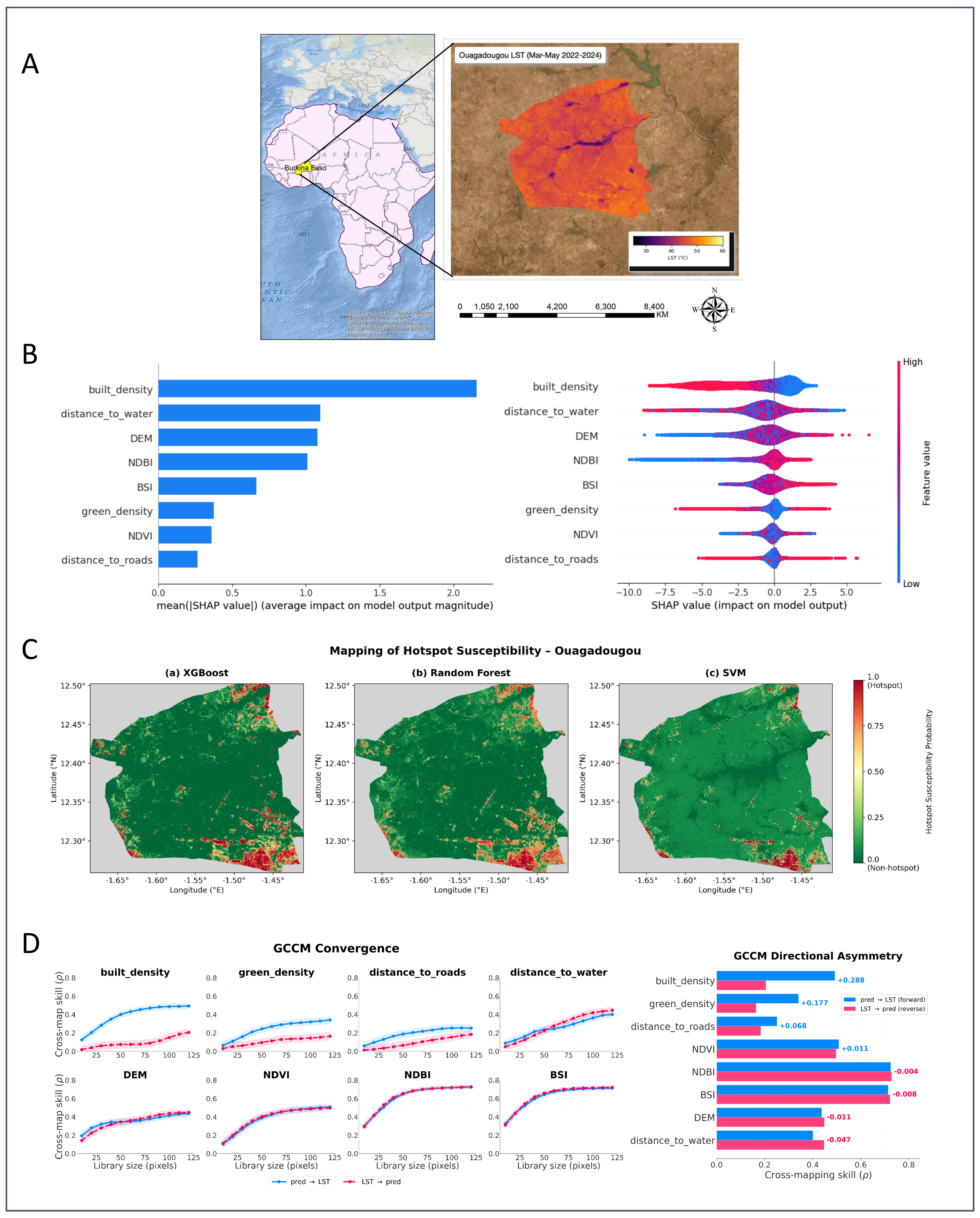
Figure 1:
A. Study area context and land surface temperature (LST) distribution across Ouagadougou during the March–May hot season (2022-2024).
B. SHAP-based global feature importance and summary distribution for the XGBoost model.
C. Spatial hotspot susceptibility maps predicted by XGBoost, Random Forest, and SVM.
D. GCCM convergence curves and directional asymmetry results.
Causal Validation (GCCM) of Predictive Features
Because several high-ranking SHAP predictors (NDBI, BSI, NDVI) share radiometric properties with thermal emission, making high correlation with LST expected but not evidence of causation, we applied GCCM to each predictor-LST pair to distinguish genuine drivers from statistical proxies. Built-up density (ρ = 0.49, 95% CI [0.46, 0.53]) and green density (ρ = 0.34 [0.30, 0.38]) showed clear unidirectional causality toward LST, with reverse cross-map skill substantially weaker (ρ = 0.21 and 0.16, respectively) and non-overlapping confidence intervals (Fig. 1D). Distance to roads also showed asymmetric coupling (ρ = 0.25 vs. 0.18), though with overlapping CIs.
In contrast, the spectral indices that ranked highly in the ML model (NDBI, BSI, NDVI; ρ = 0.50-0.73) exhibited symmetric bidirectional coupling, indicating strong association but no identifiable causal direction. Distance to water similarly showed bidirectional coupling (ρ ≈ 0.40-0.45 both ways). All predictors exhibited robust convergence (Kendall’s τ ≥ 0.94, p < 10⁻⁶).
Discussion
Hotspot formation during Ouagadougou’s March-May 2024 heatwave season was dominated by built-up density, followed by distance to water, elevation, and NDBI. GCCM confirmed unidirectional causal influence for built-up density and green density driving LST, while NDBI and BSI showed bidirectional coupling. Applying the methodology by Hoang et al., 2025 to semi-arid Ouagadougou revealed a climate-dependent reversal: sparse built-up cover increased hotspot risk, contrary to tropical Da Nang, Vietnam. In Ouagadougou, unbuilt land is predominantly bare soil with high solar absorptivity and negligible evapotranspiration Oke et al., 2017 Offerle et al., 2005, not the vegetated surfaces displaced by urbanisation in temperate climates. Denser construction reduces exposed ground through mutual shading Abedrabboh et al., 2025, while urban proximity to the central reservoir amplifies evaporative cooling Lindén, 2011, reversing the typical UHI patterns observed in other climates Hoang et al., 2025 Yeboah et al., 2025. Taken together, these results caution against generalising UHI frameworks across bioclimatic contexts and, in the context of Ouagadougou, point toward compact development and water body preservation as locally appropriate heat mitigation strategies for urban planners.
Limitations
The intra-urban heat hotspot threshold (LST > μ + 1σ) is study-relative and not anchored to health-relevant exposure limits; sensitivity to alternative thresholds (e.g., fixed percentile or absolute temperature) is untested. The random pixel-level train-test split does not account for spatial autocorrelation among neighbouring pixels, so reported F1 and Cohen’s κ likely overestimate spatial transferability. Hyperparameter selection via GridSearchCV used overall accuracy as the scoring criterion despite the 10.3% minority-class imbalance, which may have suboptimally weighted minority-class performance; class weighting and resampling strategies were not explored. The LST target is a three-year hot-season median composite, so predictor rankings may shift under interannual variability or heatwave-specific conditions not captured by seasonal aggregation. The GCCM-inferred causal directionality is supported at the 150 m neighborhood scale at which the analysis was conducted and should not be extrapolated without further evaluation to coarser spatial aggregates, other Sahelian cities, or different soil and morphological contexts.
Code and data availability
All analysis code, processing notebooks, and instructions for reproducing the figure are openly available at https://
Supplementary material
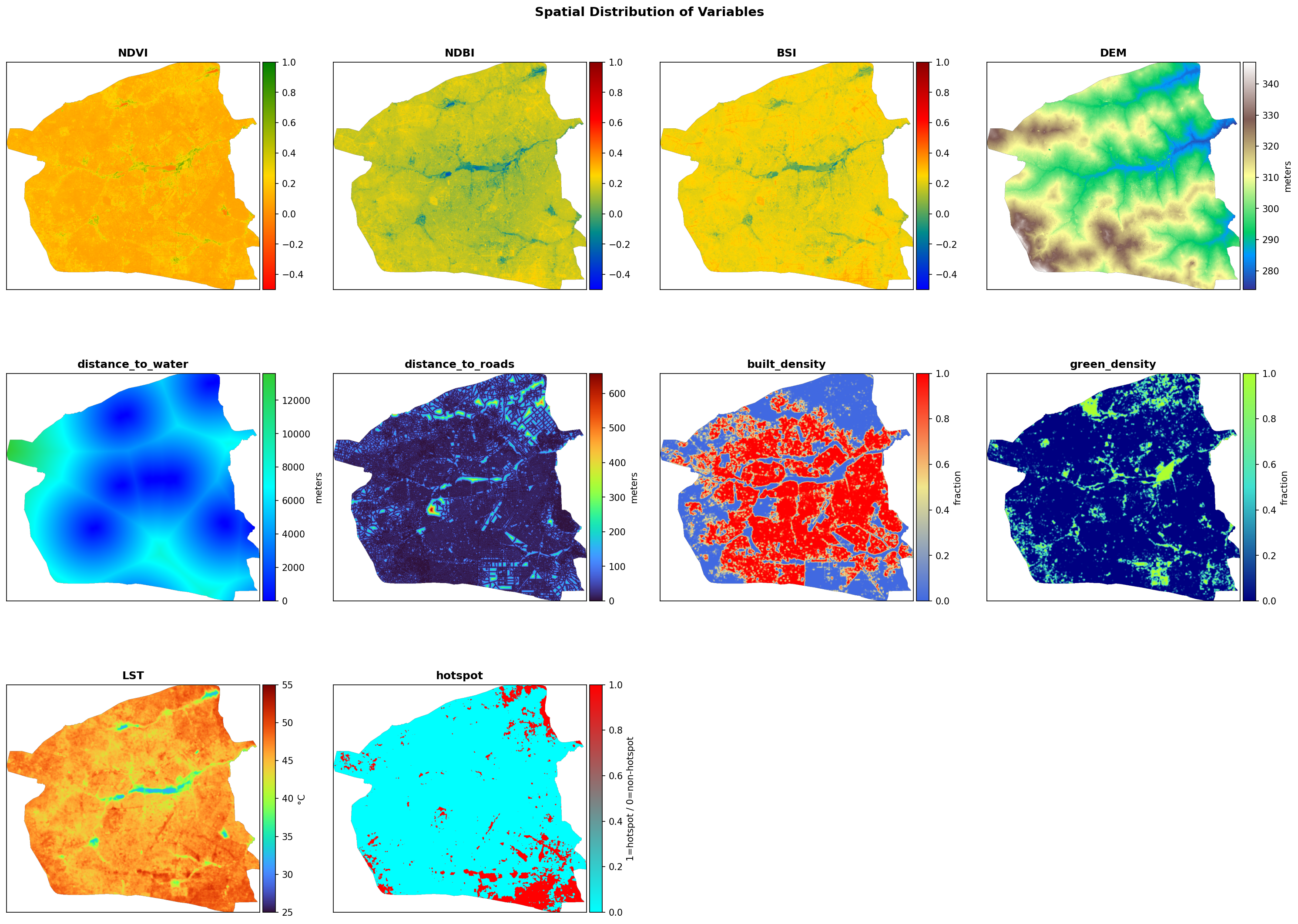
Figure 2:Spatial distribution of the ten variables (NDVI, NDBI, BSI, DEM, distance to water, distance to roads, built-up density, green space density, LST, hotspot label) across the Ouagadougou administrative boundary at 30 m resolution, March-May 2022-2024 hot-season composite.
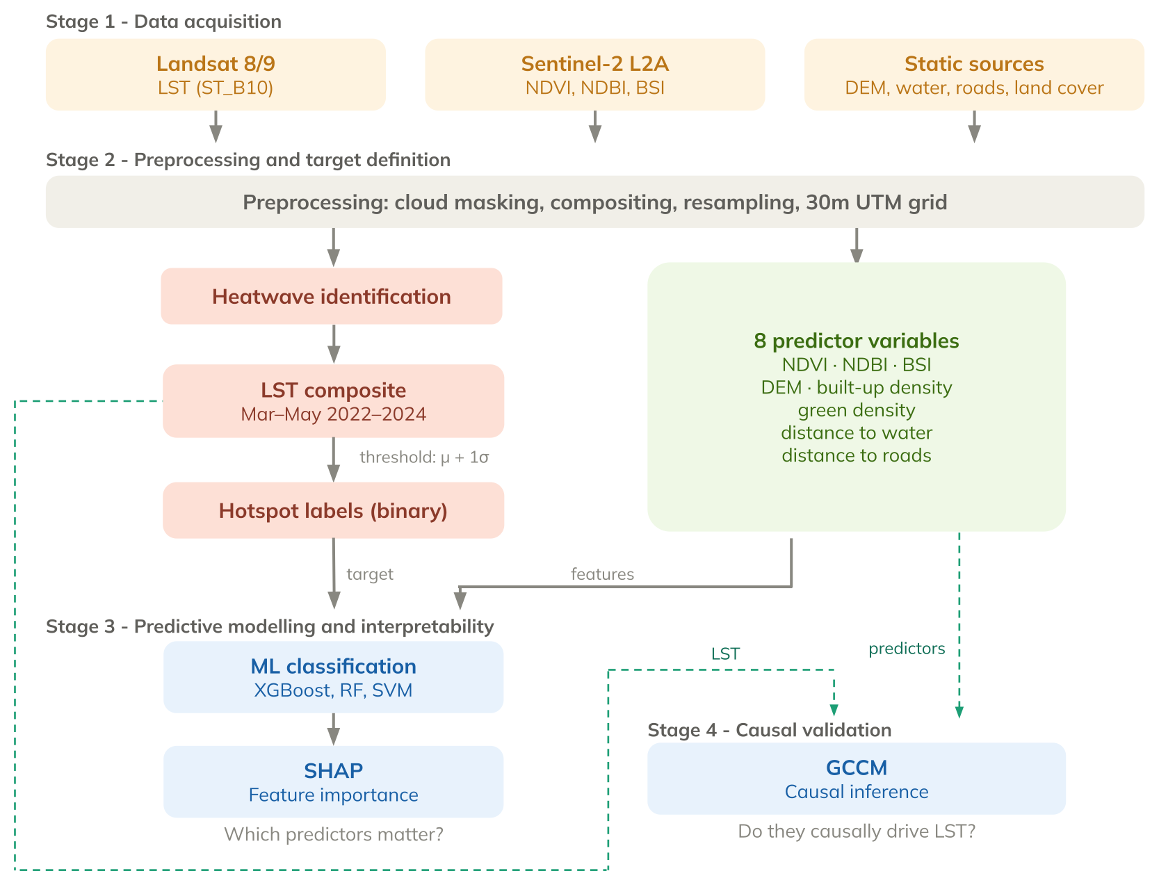
Figure 3:Methods workflow showing the four analytical stages: data acquisition, preprocessing and target definition, predictive modelling and interpretability, and causal validation.
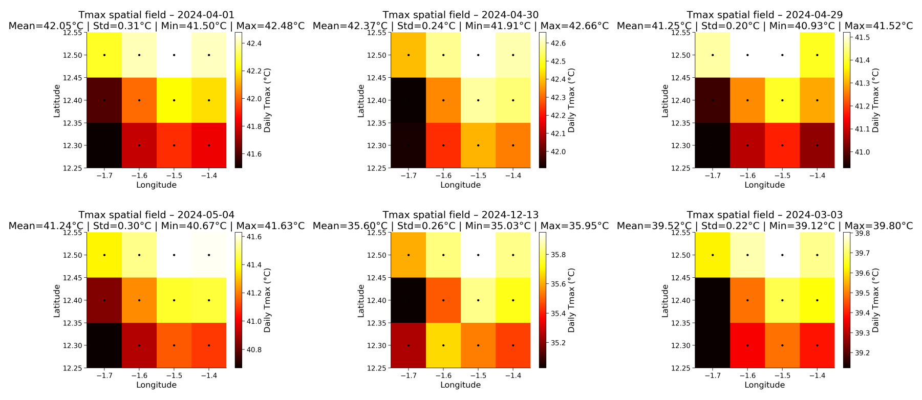
Figure 4:Six representative heatwave-event days in 2024 showing daily Tmax spatial fields across the Ouagadougou region (gridded ERA5 reanalysis, ~31 km native resolution).
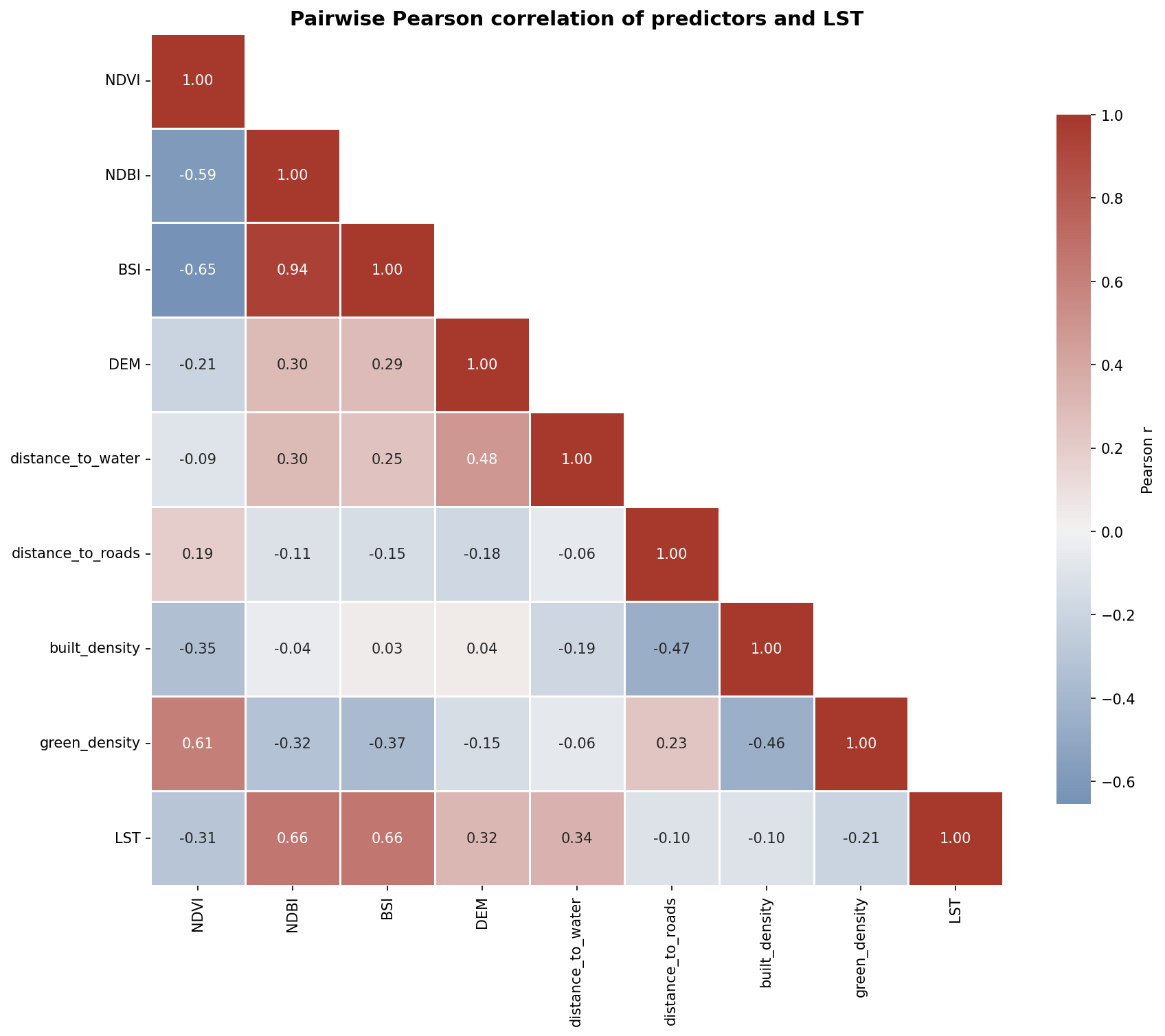
Figure 5:Pairwise Pearson correlation among the eight continuous predictors and LST. Complements Table 3 in the main text by showing all off-diagonal pairs (e.g., the high collinearity between BSI and NDBI, r ≈ +0.94).
Model hyperparameters. Selected hyperparameters for the three classifiers, read directly from the pre-fit pickled estimators archived on Zenodo (DOI: Lindner et al. (2026)).
| Hyperparameter | XGBoost | Random Forest | SVM |
|---|---|---|---|
n_estimators | 500 | 300 | — |
max_depth | 9 | none | — |
learning_rate | 0.2 | — | — |
reg_alpha | 0 | — | — |
reg_lambda | 0.001 | — | — |
C | — | — | 100 |
kernel | — | — | rbf |
gamma | — | — | scale |
probability | — | — | true |
random_state | 42 | 42 | — |
Test-set classification metrics.
| Model | Accuracy | Precision | Recall | F1 | Cohen’s κ |
|---|---|---|---|---|---|
| XGBoost | 0.946 | 0.812 | 0.616 | 0.700 | 0.671 |
| Random Forest | 0.938 | 0.866 | 0.471 | 0.610 | 0.580 |
| SVM | 0.919 | 0.806 | 0.274 | 0.408 | 0.376 |
Acknowledgments
We are grateful to the Climatematch Impact Scholars Program for providing the framework, training, and platform that made this collaboration possible. We also acknowledge the “NSF Science and Technology Center (STC) Learning the Earth With Artificial Intelligence and Physics (LEAP)” for making its Pangeo JupyterHub available to Impact Scholars participants.
Data Availability
Published via Impact Scholars; original development repository.
- Tuholske, C., Caylor, K., Funk, C., Verdin, A., Sweeney, S., Grace, K., Peterson, P., & Evans, T. (2021). Global Urban Population Exposure to Extreme Heat. Proceedings of the National Academy of Sciences, 118(41), e2024792118. 10.1073/pnas.2024792118
- Seto, K. C., Güneralp, B., & Hutyra, L. R. (2012). Global Forecasts of Urban Expansion to 2030 and Direct Impacts on Biodiversity and Carbon Pools. Proceedings of the National Academy of Sciences, 109(40), 16083–16088. 10.1073/pnas.1211658109
- Voogt, J. A., & Oke, T. R. (2003). Thermal Remote Sensing of Urban Climates. Remote Sensing of Environment, 86(3), 370–384. 10.1016/S0034-4257(03)00079-8
- Pekel, J.-F., Cottam, A., Gorelick, N., & Belward, A. S. (2016). High-resolution mapping of global surface water and its long-term changes. Nature, 540(7633), 418–422. 10.1038/nature20584
- Gao, B., Yang, J., Chen, Z., Sugihara, G., Li, M., Stein, A., Kwan, M.-P., & Wang, J. (2023). Causal inference from cross-sectional earth system data with geographical convergent cross mapping. Nature Communications, 14, 5875. 10.1038/s41467-023-41619-6
- Hoang, N.-D., Huynh, T.-C., & Bui, D.-T. (2025). An Interpretable Machine Learning Framework for Mapping Hotspots and Identifying Their Driving Factors in Urban Environments during Heat Waves. Environmental Monitoring and Assessment, 197, 1017. 10.1007/s10661-025-14461-0
- Oke, T. R., Mills, G., Christen, A., & Voogt, J. A. (2017). Urban Climates. Cambridge University Press. 10.1017/9781139016476
- Weng, Q., Lu, D., & Schubring, J. (2004). Estimation of land surface temperature-vegetation abundance relationship for urban heat island studies. Remote Sensing of Environment, 89(4), 467–483. 10.1016/j.rse.2003.11.005
- Chen, T., & Guestrin, C. (2016). XGBoost: A Scalable Tree Boosting System. Proceedings of the 22nd ACM SIGKDD International Conference on Knowledge Discovery and Data Mining, 785–794. 10.1145/2939672.2939785
- Breiman, L. (2001). Random Forests. Machine Learning, 45(1), 5–32. 10.1023/A:1010933404324
- Lundberg, S. M., & Lee, S.-I. (2017). A Unified Approach to Interpreting Model Predictions. Advances in Neural Information Processing Systems, 30, 4765–4774.
- Lv, W. (2025). spEDM: Spatial Empirical Dynamic Modeling (R package version 1.7). 10.32614/CRAN.package.spEDM
- Sugihara, G., May, R., Ye, H., Hsieh, C., Deyle, E., Fogarty, M., & Munch, S. (2012). Detecting causality in complex ecosystems. Science, 338(6106), 496–500. 10.1126/science.1227079
- Landis, J. R., & Koch, G. G. (1977). The Measurement of Observer Agreement for Categorical Data. Biometrics, 33(1), 159–174. 10.2307/2529310
- Tang, Y., Zhang, Y.-Q., Chawla, N. V., & Krasser, S. (2009). SVMs Modeling for Highly Imbalanced Classification. IEEE Transactions on Systems, Man, and Cybernetics, Part B (Cybernetics), 39(1), 281–288. 10.1109/TSMCB.2008.2002909