A Brain-Wide Atlas of Intrinsic Neural Timescales in Mice
Abstract
Understanding how the brain integrates information requires a shift from localized functional studies to mapping a brain-wide temporal architecture. Intrinsic neural timescales (ITs), defined as the decay time constant of a neuron’s spontaneous spiking autocorrelation, provide a quantitative proxy for how long a local circuit retains information about its recent activity. Yet their accurate estimation has historically been limited by computational biases in spike train analysis and the oversimplified assumption that each neuron operates on a single characteristic timescale. In this study, we address these limitations by applying a hybrid framework combining the unbinned intrinsic Spike Time Tiling Coefficient (iSTTC) autocorrelation estimator with Bayesian Information Criterion (BIC)-guided multi-exponential modeling to 89,047 single units across 266 mouse brain regions. We reveal a robust rostro-caudal hierarchy of intrinsic neural timescales across 220 mouse brain regions, with median effective timescales approximately 4.5-fold longer in the hindbrain (956 ms) than in the forebrain (213 ms), establishing anatomical location as a key determinant of a neuron’s temporal integration window. We further demonstrate that 73.9% of neurons are better described by multi-component models, and find that fast () and slow () dynamical modes co-vary sublinearly across regions. These findings lay the groundwork for future analyses linking single-neuron dynamics to the emergence of stable, population-level representations required for decision making and adaptive behavior.
Introduction
Intrinsic neural timescales () describe how long neuronal activity remains correlated with its own past. Fast (short-) regions respond rapidly to sensory inputs, while slow (long-) regions sustain activity across delays, supporting evidence accumulation and memory Murray et al. (2014)Wasmuht et al. (2018). Quantified as the decay time constant of spontaneous spiking autocorrelation, intrinsic neural timescales have emerged as a fundamental metric of this process Murray et al. (2014). Longer timescales are thought to underlie cognitive computations that require information to be maintained over time, including working memory, evidence accumulation, and decision making.
However, constructing a brain-wide map of timescales presents significant methodological challenges. Classical binned autocorrelation functions (ACFs) systematically underestimate timescales for neurons with low firing rates or bursty dynamics, conditions common across subcortical and hindbrain regions. Furthermore, fitting a single exponential decay assumes each neuron operates on only one characteristic timescale, obscuring the multi-component temporal architecture present in the majority of neurons. To address both limitations, we apply the intrinsic Spike Time Tiling Coefficient (iSTTC), an unbinned estimator that computes autocorrelations directly from exact spike times, alongside Bayesian Information Criterion (BIC)-guided multi-exponential modeling. This combination enables reliable timescale estimation in low-firing neurons and captures multi-component temporal structure across 86% of mouse brain regions.
The IBL dataset is uniquely suited for this analysis: its brain-wide Neuropixels coverage and standardized 5–10-minute spontaneous activity recordings enable timescale estimation across nearly all major brain structures.
Methods
We analyzed 580,598 units from the IBL 2025 Brainwide Map Release International Brain Laboratory et al. (2025) during 5–10-minute spontaneous epochs. Units with ≥100 spikes, declining autocorrelations, and fit ≥ 0.5 were retained (89,047 units, 15.34%). Brain regions were grouped using the Beryl parcellation — a brain-wide region atlas developed by the International Brain Laboratory (n.d.) — into major divisions (forebrain, midbrain, hindbrain), 12 subdivisions, and 266 individual regions (220 with ≥15 neurons analyzed).
Timescales were estimated using iSTTC, an unbinned autocorrelation estimator operating on exact spike times Pochinok et al. (2026), avoiding biases in low-firing-rate neurons. Unlike binned ACF methods, iSTTC estimates are insensitive to bin size and epoching artifacts (Supplementary Figure 1). Each autocorrelation was fitted with 1–4 exponential components:
with optimal component count selected by BIC (≥1% contribution each). This revealed that 73.9% of neurons exhibit multiple timescales: a fast component () and slow component (). The amplitude-weighted effective timescale summarizes overall temporal persistence. Full details in Supplementary Methods.
Results
After quality filtering (see Methods), 89,047 units (15.3% of recorded units) across 220 regions (71% of the Beryl parcellation; ≥15 neurons each) were retained for analysis (Supplementary Figure 2).
A clear anatomical gradient emerged when neurons were grouped by major division. The forebrain exhibited the shortest timescales (median = 213 ms, IQR = 120–304 ms), while the midbrain and hindbrain showed markedly longer temporal persistence (765 ms, IQR = 482–968 ms and 956 ms, IQR = 723–1183 ms, respectively) (Figure 1A). This forebrain-to-hindbrain organisation was further reflected at the level of individual Beryl subdivisions, with hippocampal and cortical subplate regions anchoring the fast end and hindbrain nuclei clustering at the slow extreme (Figure 1B) International Brain Laboratory (n.d.).
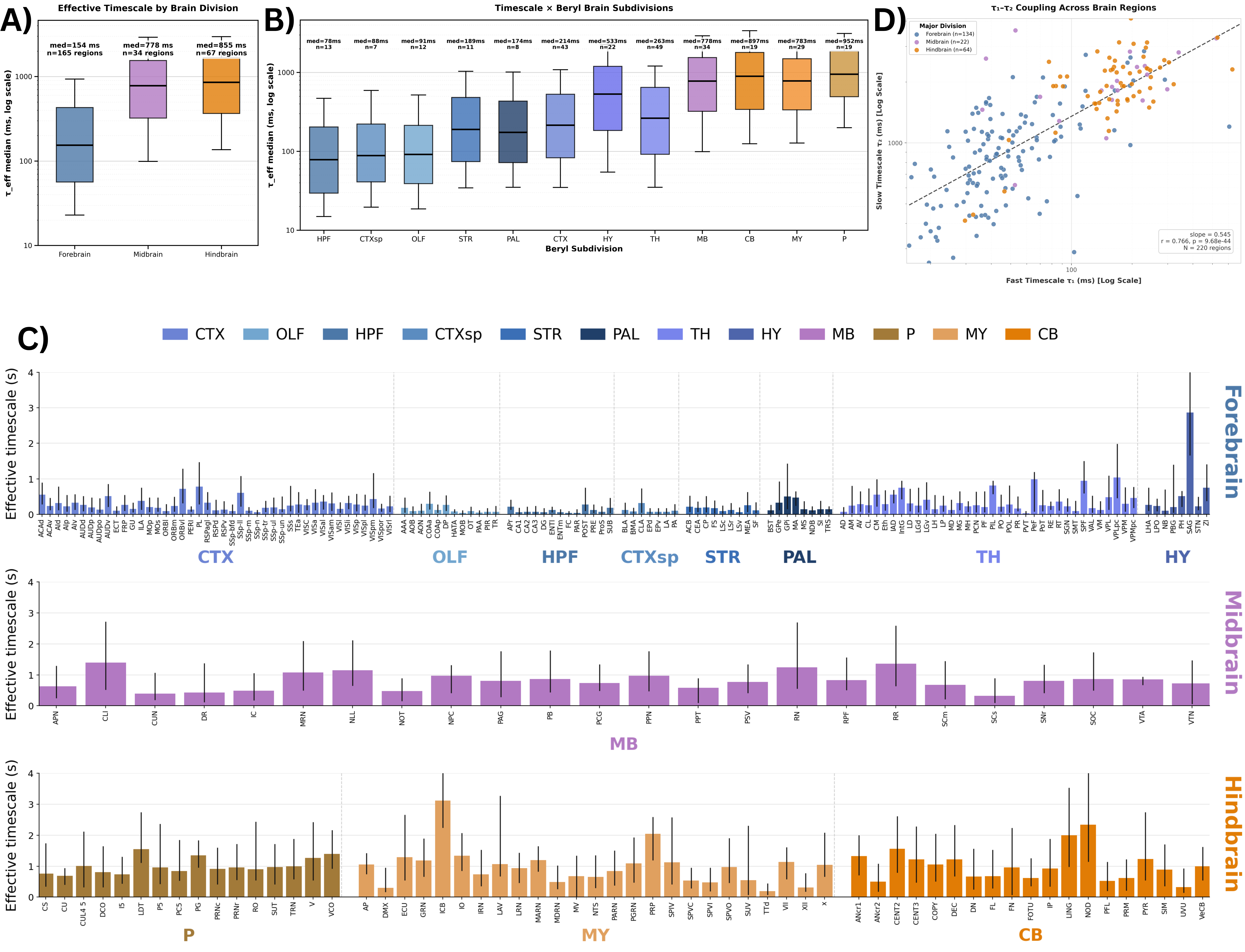
Figure 1:Brain-wide map of intrinsic neural timescales across brain regions. All panels except C exclude regions with fewer than 15 neurons (220 regions retained); C excludes regions with fewer than 5 neurons (244 regions retained). (A) Effective timescale distributions by major brain division (forebrain, midbrain, hindbrain); boxes show the interquartile range of region-level medians, with whiskers extending to the 10th and 90th percentiles. (B) Timescale distributions across the 12 Beryl parcellation subdivisions, ordered from fastest to slowest median . Boxes show the interquartile range and whiskers indicate the 10th and 90th percentiles. (C) Brain-wide bar chart of median per region; bars show median and error bars indicate the interquartile range (Q1–Q3). Regions are grouped by major anatomical division — forebrain (top), midbrain (middle), and hindbrain (bottom) — and ordered alphabetically within each subdivision. Colour denotes Allen Mouse Brain Atlas Beryl parcellation subdivision (CTX, isocortex; OLF, olfactory areas; HPF, hippocampal formation; CTXsp, cortical subplate; STR, striatum; PAL, pallidum; TH, thalamus; HY, hypothalamus; P, pons; MY, medulla; MB, midbrain; CB, cerebellum). (D) Coupled multiscale architecture of fast and slow timescale components. Each point represents one brain region ( = 220 regions with reliable two-component fits), plotted by its median fast timescale () against its median slow timescale () on log-log axes. Colors denote major division: forebrain, midbrain, and hindbrain. The dashed line shows the log-log regression fit (slope = 0.545, = 0.766, = 9.68 × 10⁻⁴⁴), indicating that regions with longer fast timescales also tend to have proportionally longer slow timescales.
Median spanned nearly two orders of magnitude, ranging from 37.9 ms in the paraventricular nucleus of the thalamus to 3,115 ms in the infracerebellar nucleus (Figure 1C). Despite this striking gradient, the remaining ~79% of timescale variance reflected variability within regions (median IQR = 588 ms per area) (Supplementary Figure 3), highlighting that anatomical region is a meaningful but partial determinant of a neuron’s temporal dynamics.
Results were consistent across a Bayesian hierarchical model controlling for mouse, session, and probe ( = 77,058 neurons, 131 mice; Supplementary Methods), which confirmed brain region as the dominant source of variance (24.1%), with mouse identity accounting for only 2.3%, confirming the gradient reflects anatomical organisation rather than inter-individual differences (Supplementary Table 1). This gradient was independent of firing rate (Supplementary Figure 4). Posterior estimates strongly supported longer intrinsic timescales in midbrain and hindbrain relative to forebrain (forebrain < midbrain, ; forebrain < hindbrain, ; = posterior probability of violation), while largely preserving the subdivision-level ordering (Spearman = 0.895, < 0.001). Notably, the 24.1% of variance attributable to brain region is nearly an order of magnitude higher than the 2.5% reported by Shi et al. (2025), who analyzed an earlier version of the IBL dataset with 11,468 neurons. The source of this discrepancy warrants further investigation.
73.9% of neurons required multi-component models (Supplementary Figure 5), raising the question of whether fast and slow components are independently organized or jointly constrained. We therefore examined how co-varies with across regions, restricting the analysis to neurons best described by exactly two components (60.4%). In this model, and correspond to the faster (shorter) and slower (longer) time constants, respectively. co-varied strongly with (Pearson = 0.766, = 9.68 × 10⁻⁴⁴; Figure 1D), as assessed via ordinary least-squares linear regression on log-transformed region-level medians, following a sublinear relationship (slope = 0.545 on log-log axes), indicating that regions with longer fast timescales also tend to have proportionally longer slow timescales.
Discussion
Our central finding is that anatomical position along the rostro-caudal axis is a strong organisational principle of intrinsic neural timescales in mice, a hierarchy that holds robustly across 220 regions in the largest single-dataset mapping effort to date. The longer timescales of midbrain and hindbrain structures may reflect their roles in integrating homeostatic, motor, and state-related signals over extended periods, such as during decision-making Grill & Hayes (2012)Caggiano et al. (2018). Critically, this hierarchy is not merely a population-level abstraction: among 56 mice contributing neurons to at least four Beryl subdivisions, every individual animal showed shorter forebrain than hindbrain timescales, with within-mouse rank orderings correlating strongly with the population-level gradient (median Spearman = 0.76, ), demonstrating that the rostro-caudal timescale hierarchy is a robust and consistent feature of individual mouse brains.
The majority of neurons exhibit multiple timescale components, with fast () and slow () dynamical modes co-varying sublinearly across brain regions. While these fitted components reflect statistically distinguishable decay regimes, they likely emerge from distinct biological substrates. Nevertheless, the two components may have partially separable origins. Cortical and hippocampal values (30 ms and 18 ms, respectively) fall within the range of intracellularly measured membrane time constants McCormick et al. (1985)Spruston & Johnston (1992), suggesting may primarily reflect intrinsic neuronal properties and fast local inhibitory kinetics. By contrast, values extending to several seconds exceed any known single-neuron biophysical timescale, pointing instead to recurrent network interactions or neuromodulatory processes. The observed sublinear compression of relative to aligns with this interpretation, indicating interacting but distinct cellular and circuit-level constraints Chaudhuri et al. (2015).
The substantial within-region variance in (median IQR = 588 ms per area) warrants attention in future work. Regional medians may obscure meaningful neuron-to-neuron heterogeneity that is functionally relevant, motivating analyses of full timescale distributions within regions rather than summary statistics alone. This within-region variance likely reflects unmeasured factors including cell type, laminar position, and local connectivity, which future work integrating timescale estimates with molecular or anatomical cell-type information could resolve. More broadly, the multi-timescale architecture we describe provides a framework for linking single-neuron dynamics to population-level computation, and for testing whether the balance between fast and slow dynamical modes shapes the stability of neural representations during decision-making.
Limitations
While our hybrid approach resolves key biases, some limitations remain. Estimating ultra-slow timescales ( > 2,000 ms) yields wide confidence intervals due to the inherent limit of the ~10-minute recording epoch. Additionally, regions dominated by highly regular oscillatory dynamics (such as theta rhythms in the hippocampus) exhibited lower fit qualities (), as sum-of-exponentials models cannot fully capture non-monotonic ACF structures.
Because intrinsic timescales were estimated from the full spontaneous epoch, early passive-state transients may contribute to the estimates. When the passive period begins, the mouse has just finished performing the decision-making task, and residual task-related signals may persist for tens of seconds into the passive epoch, potentially biasing upward in regions strongly recruited by the task. Future robustness analyses should test whether excluding the first 60–120 s of spontaneous activity changes the observed anatomical hierarchy.
Supplementary Methods
Dataset and unit selection. We analyzed spontaneous spiking activity from 580,598 recorded units across 427 sessions, 651 probes, 131 mice, and 266 brain regions using the open-access IBL 2025 Brainwide Map Release International Brain Laboratory et al. (2025) Neuropixels dataset, focusing on the 5–10-minute passive resting state epochs for computing intrinsic timescales.
Units were retained for analysis if they met all of the following quality criteria: ≥100 spontaneous spikes, a declining iSTTC autocorrelation in the 50–200 ms window, multi-exponential fit ≥ 0.5, 95% confidence interval of excluding zero, and below the upper bound of the exponential fitting range (30,000 ms), which would indicate a failed rather than converged estimate. Following these criteria, 89,047 viable units (representing 15.34% of the initial population) were retained for downstream analysis.
Rationale for unit quality criteria. Our quality filtering criteria were designed to ensure reliable intrinsic timescale estimation while preserving broad anatomical coverage. Each criterion addressed a specific methodological concern:
Minimum spike count (≥100 spikes): This threshold follows prior intrinsic timescale studies Murray et al. (2014)Wasmuht et al. (2018)Shi et al. (2025). Reliable autocorrelation estimation requires sufficient spike counts; units with fewer than 100 spikes during the spontaneous epoch produce noisy autocorrelation functions and unstable timescale estimates with large confidence intervals.
Declining autocorrelation (50–200 ms window): Units whose autocorrelation functions failed to decline within this range violated the assumption that intrinsic timescales reflect temporal decay. Non-declining autocorrelations often indicate oscillatory activity, recording artifacts, or multi-unit contamination, all of which produce unstable exponential fits.
Minimum fit quality ( ≥ 0.5): This criterion ensured that the sum-of-exponentials model adequately captured autocorrelation structure. Low values typically reflected oscillatory or irregular firing patterns, or insufficient data for reliable fitting.
Bounded confidence intervals and convergence: Requiring the 95% confidence interval of to exclude zero and to remain below the fitting upper bound (30,000 ms) excluded poorly constrained or non-convergent estimates that would otherwise introduce noise into downstream analyses.
iSTTC estimator. iSTTC estimates the autocorrelation-like function by generating temporally shifted copies of each spike train and computing the Spike Time Tiling Coefficient (STTC) between the original and shifted versions at successive lags ( = 5 ms, 600–1200 lags). Because STTC operates directly on exact spike times rather than binned counts, it is insensitive to zero-padding artifacts and does not require a minimum firing rate threshold. We confirmed that iSTTC-derived estimates showed no systematic dependence on firing rate across the analyzed population (Supplementary Figure 4), ensuring that the observed timescale distributions reflect genuine temporal integration properties rather than sampling biases.
iSTTC derivation. The iSTTC is an extension of the Spike Time Tiling Coefficient Cutts & Eglen (2014), adapted to estimate autocorrelation directly from non-binned spike times Pochinok et al. (2026). The standard STTC between two spike trains A and B is:
where () is the proportion of recording length within of any spike in train A (B), and () is the proportion of spikes in A (B) falling within of any spike in B (A). For autocorrelation estimation, lagged copies of each spike train are generated by shifting the original train by lag , with both copies truncated to span equal durations. The iSTTC at lag is computed using the same STTC formula applied to these aligned, truncated trains, yielding an unbinned autocorrelation curve per neuron.
Multi-exponential model fitting and component selection. Each neuron’s iSTTC autocorrelation curve was fitted with = 1–4 exponential decay components:
The optimal was selected by minimising the Bayesian Information Criterion:
where ( amplitudes and time constants), is the number of lag points, and is the maximised likelihood under Gaussian residuals. Following Shi et al. (2025), each component was required to contribute at least 1% to the total autocorrelation shape; if a more complex model was preferred by BIC but violated this constraint, the simpler model was retained. The amplitude-weighted effective timescale was computed from the selected model. For the – coupling analysis, neurons with three or more components (13.8%) were excluded, as the small number per region precluded stable regional estimates.
Bayesian hierarchical model and variance decomposition. To provide a principled decomposition of variance across the data hierarchy and to test whether the anatomical gradient persisted after accounting for inter-individual differences, we fitted a Bayesian hierarchical model using PyMC (NUTS sampler, 4 chains, 2000 posterior draws, 1000 warmup iterations). The model predicted using random intercepts for Beryl region, mouse, session, and probe, with weakly informative half-normal priors placed on all variance components. All parameters converged successfully (all ≤ 1.02, 0 divergences). Variance shares were computed from posterior mean standard deviations as . Posterior probabilities of direction (e.g. forebrain < midbrain) were computed as the fraction of posterior samples in which the inequality was violated.
Within-mouse consistency. For each mouse with neurons in at least four Beryl subdivisions ( = 56), we computed the Spearman rank correlation between its per-subdivision median and the population-level ordering, tested against zero via one-sample t-test.
Supplementary Figures
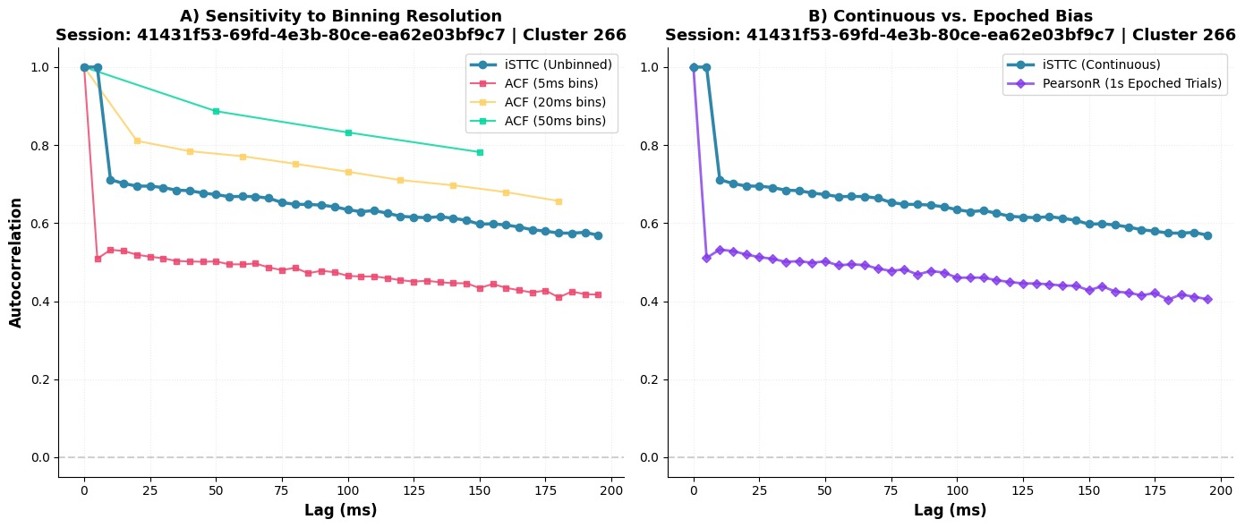
Supplementary Figure 1: Methodological comparison of autocorrelation estimators for a representative neuron. Results shown for an example neuron (Session 41431f53, Cluster 266) to illustrate the sensitivity of autocorrelation estimates to methodological choices. (A) Sensitivity to binning resolution: binned ACF estimates vary substantially depending on bin size (5 ms, 20 ms, 50 ms bins), while iSTTC (unbinned) provides a consistent estimate independent of bin size. (B) Continuous vs. epoched bias: iSTTC on the continuous spike train yields a higher and more slowly decaying autocorrelation than PearsonR on 1s epoched trials, illustrating that trial-based epoching can introduce a downward bias. These examples motivate the use of iSTTC for timescale estimation; systematic validation across the full population is provided in Supplementary Figure 4.
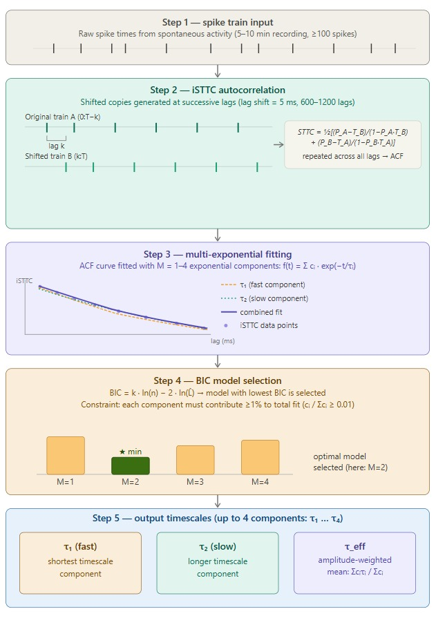
Supplementary Figure 2: Pipeline for estimating intrinsic neural timescales using iSTTC. Raw spike times from spontaneous activity recordings (5–10 min, ≥100 spikes) are processed in five steps: (1) spike train input; (2) iSTTC autocorrelation, computed by generating shifted copies of each spike train at successive lags (lag shift = 5 ms, 600–1200 lags) and applying the STTC formula to produce an autocorrelation curve; (3) multi-exponential fitting with = 1–4 components; (4) BIC model selection, with the constraint that each component contributes ≥1% to the total fit; (5) output timescales – and amplitude-weighted effective timescale .
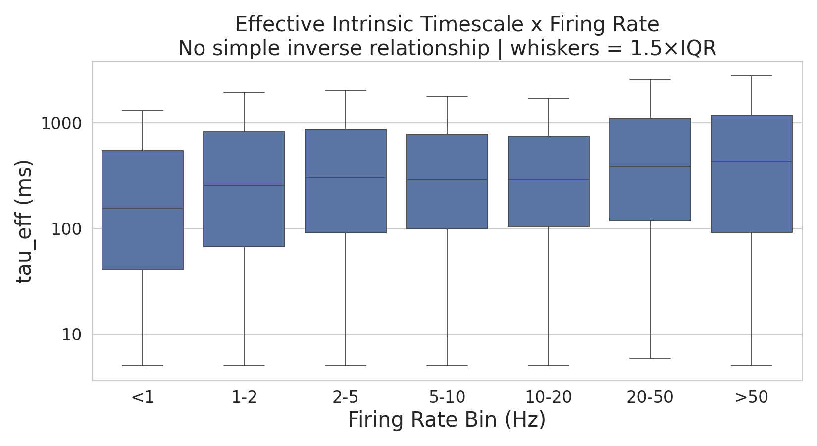
Supplementary Figure 3: Effective intrinsic timescale as a function of firing rate. Distribution of across neurons grouped into firing rate bins (IQR shown as box height, median as horizontal line, log scale on both axes). Contrary to the expectation that high firing rates would trivially produce short timescales, no simple inverse relationship is observed: median is lowest in the <1 Hz bin and rises across intermediate firing rates, with the highest median values in the 20–50 and >50 Hz bins. The broad IQR within each bin further indicates that firing rate is a poor predictor of at the single-neuron level.
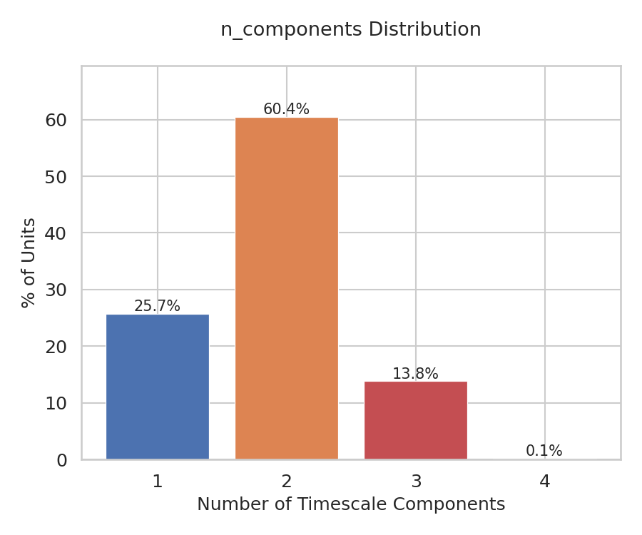
Supplementary Figure 4: Distribution of the number of timescale components per neuron. The majority of well-fitted neurons were best described by two-timescale models (60.4%), followed by one-timescale (25.7%) and three-timescale (13.8%) models, with only 0.1% requiring four timescales. The optimal number of components was selected using the Bayesian information criterion (BIC), with the constraint that each component contributed at least 1% to the overall autocorrelation shape.
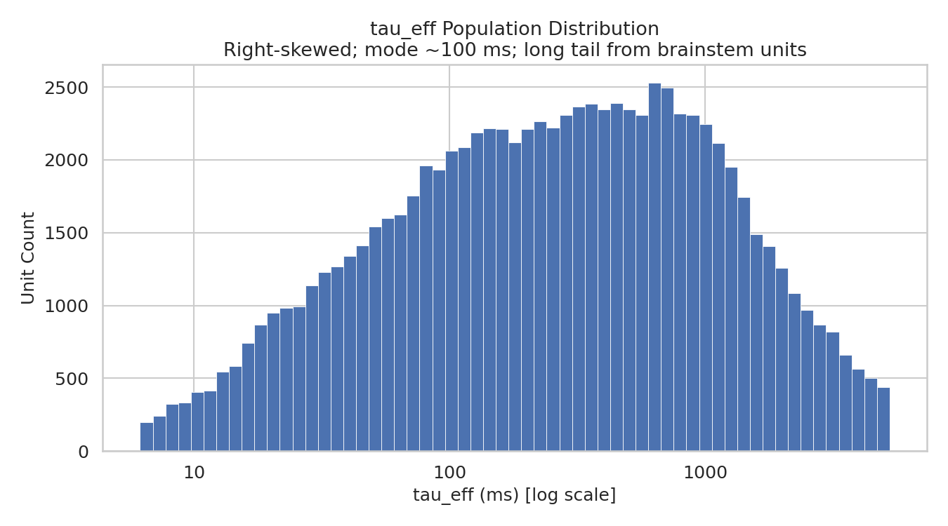
Supplementary Figure 5: Population distribution of effective intrinsic timescales. Histogram of across all well-fitted neurons (log-scaled x-axis), revealing a broad, right-skewed distribution with a mode near 800 ms and a heavy tail extending beyond 1,000 ms.
Supplementary Tables
Supplementary Table 1: Bayesian variance decomposition. Proportion of variance in attributable to each level of the data hierarchy, estimated simultaneously from a Bayesian hierarchical model with random intercepts for brain region, mouse, session, and probe (PyMC, NUTS sampler, 4 chains, 2000 draws; all ≤ 1.02, 0 divergences). Variance shares computed from posterior mean standard deviations as . Credible intervals are 89% highest density intervals (HDI) following ArviZ defaults. Brain region is the dominant source of structured variance, with mouse identity accounting for a comparatively small share, indicating that inter-individual differences largely reflect differences in anatomical sampling.
| Source | Variance (%) | 89% HDI (%) |
|---|---|---|
| Brain region | 24.1 | 20.4–28.1 |
| Mouse | 2.3 | 1.2–3.5 |
| Session | 5.0 | 3.5–7.0 |
| Probe | 7.0 | 6.2–7.9 |
| Neuron residual | 61.6 | — |
Acknowledgments
Supported by Neuromatch Impact Scholars Program. Data from International Brain Laboratory 2025 Brainwide Map Release. We thank the IBL consortium for open data access and Jason Manley for supervision. Analysis builds on iSTTC methodology Pochinok et al. (2026) and multi-exponential fitting framework Shi et al. (2025).
Data Availability
Published via Impact Scholars; original development repository.
- Murray, J. D., Bernacchia, A., Freedman, D. J., Romo, R., Wallis, J. D., Cai, X., Padoa-Schioppa, C., Pasternak, T., Seo, H., Lee, D., & Wang, X.-J. (2014). A Hierarchy of Intrinsic Timescales across the Primate Cortex. Nature Neuroscience, 17, 1661–1663. 10.1038/nn.3862
- Wasmuht, D. F., Spaak, E., Buschman, T. J., Miller, E. K., & Stokes, M. G. (2018). Intrinsic Neuronal Dynamics Predict Distinct Functional Roles during Working Memory. Nature Communications, 9, 3499. 10.1038/s41467-018-05961-4
- International Brain Laboratory, Angelaki, D. E., Benson, B., & others. (2025). A Brain-Wide Map of Neural Activity during Complex Behaviour. Nature, 645, 177–191. 10.1038/s41586-025-09235-0
- International Brain Laboratory. (n.d.). iblatlas.regions: IBL Library Documentation. https://docs.internationalbrainlab.org/_autosummary/iblatlas.regions.html
- Pochinok, I., Hanganu-Opatz, I. L., & Chini, M. (2026). iSTTC: A Robust Method for Accurate Estimation of Intrinsic Neural Timescales from Single-Unit Recordings. PLOS Computational Biology, 22(3), e1013385. 10.1371/journal.pcbi.1013385
- Shi, Y.-L., Zeraati, R., International Brain Laboratory, Levina, A., & Engel, T. A. (2025). Brain-Wide Organization of Intrinsic Timescales at Single-Neuron Resolution. bioRxiv. 10.1101/2025.08.30.673281
- Grill, H. J., & Hayes, M. R. (2012). Hindbrain Neurons as an Essential Hub in the Neuroanatomically Distributed Control of Energy Balance. Cell Metabolism, 16(3), 296–309. 10.1016/j.cmet.2012.06.015
- Caggiano, V., Leiras, R., Goñi-Erro, H., Masini, D., Bellardita, C., Bouvier, J., Caldeira, V., Fisone, G., & Kiehn, O. (2018). Midbrain Circuits that Set Locomotor Speed and Gait Selection. Nature, 553, 455–460. 10.1038/nature25448
- McCormick, D. A., Connors, B. W., Lighthall, J. W., & Prince, D. A. (1985). Comparative Electrophysiology of Pyramidal and Sparsely Spiny Stellate Neurons of the Neocortex. Journal of Neurophysiology, 54(4), 782–806. 10.1152/jn.1985.54.4.782
- Spruston, N., & Johnston, D. (1992). Perforated Patch-Clamp Analysis of the Passive Membrane Properties of Three Classes of Hippocampal Neurons. Journal of Neurophysiology, 67(3), 508–529. 10.1152/jn.1992.67.3.508
- Chaudhuri, R., Knoblauch, K., Gariel, M.-A., Kennedy, H., & Wang, X.-J. (2015). A Large-Scale Circuit Mechanism for Hierarchical Dynamical Processing in the Primate Cortex. Neuron, 88(2), 419–431. 10.1016/j.neuron.2015.09.008
- Cutts, C. S., & Eglen, S. J. (2014). Detecting Pairwise Correlations in Spike Trains: An Objective Comparison of Methods and Application to the Study of Retinal Waves. Journal of Neuroscience, 34(43), 14288–14303. 10.1523/JNEUROSCI.2767-14.2014