Supplementary Information — NMDA Modulates Working Memory Attractor Stability

Supplementary Figures¶

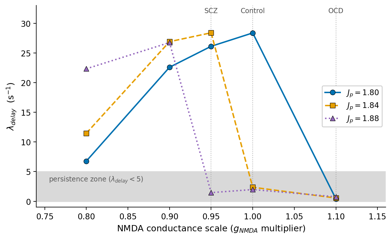
This supplement gives the complete mathematical description of the spiking network (Network model), the exact parameter values used in all simulations (Table 1–Table 4), the definition of the $\lambda_{\mathrm{delay}}$ metric (The $\lambda_{\mathrm{delay}}$ metric), the multi-seed statistical protocol (Multi-seed statistical protocol), a supplementary NMDA-conductance sweep (Figure 3), and the full statistical tables (Statistical tables). The model follows the integrate-and-fire framework of Loh et al., 2007 as used by Loh et al., 2007, and was implemented in Brian2 Stimberg et al., 2019.

Network model¶

Single-neuron dynamics¶

Both excitatory ($E$) and inhibitory ($I$) cells are leaky integrate-and-fire neurons. The subthreshold membrane potential $V$ obeys

with cell-type-specific $C_m$ and $g_L$ (Table 1). When $V$ reaches the threshold $V_{\mathrm{th}}$ a spike is emitted and $V$ is clamped to the reset $V_{r}$ for an absolute refractory period $t_{\mathrm{ref}}$. The total synaptic current is

Synaptic currents¶

AMPA (external and recurrent) and GABA$_{\mathrm A}$ currents are

where each presynaptic spike at $t_k$ increments the conductance variable by the corresponding synaptic weight. The NMDA current carries a voltage-dependent Mg$^{2+}$ block Jahr & Stevens, 1990:

with $V$ in mV and $[\mathrm{Mg}^{2+}]$ in mM. The NMDA gating variable has a two-stage (rise/decay) form,

and $s^{\mathrm{tot}}_{\mathrm{NMDA}}$ denotes the gating summed over the presynaptic excitatory pool. All synapses act with a transmission delay of $0.5\ \mathrm{ms}$.

Architecture and connectivity¶

The network contains $N=2000$ neurons: $N_E=1600$ excitatory ($f_{\mathrm{inh}}=0.20$) and $N_I=400$ inhibitory. The excitatory population is split into two selective pools $S_1$ and $S_2$ of 240 neurons each ($f_{\mathrm{sel}}=0.15$ of $N_E$) and a non-selective pool (NS) of 1120 neurons. The inhibitory pool provides global feedback inhibition. Recurrent excitation is structured by a within-pool potentiation factor $J_p$ and a compensating cross-pool factor

which keeps the mean recurrent input constant as $J_p$ varies. Excitatory–excitatory AMPA weights are $g_{\mathrm{EEA}}$ (baseline), $g_{\mathrm{EEA}}J_p$ (within a selective pool) and $g_{\mathrm{EEA}}J_m$ (between selective pools); recurrent NMDA is pooled analogously. $E -> I$, $I -> E$ and $I -> I$ connections are all-to-all with weights $g_{\mathrm{EIA}}$, $g_{\mathrm{IE}}$ and $g_{\mathrm{II}}$ respectively. Base conductances (Table 3) are calibrated for $N=2000$ and rescaled by $1600/N_E$ (excitatory) and $400/N_I$ (inhibitory) for other network sizes.

Background input and stimulation protocol¶

Every neuron receives $N_{\mathrm{ext}}=800$ independent external AMPA synapses driven by Poisson spike trains at $3\ \mathrm{Hz}$ each ($2.4\ \mathrm{kHz}$ aggregate), reproducing cortical spontaneous activity. A $200\ \mathrm{ms}$ spontaneous period is followed by a cue of $200\ \mathrm{Hz}$ applied to $S_1$ over $t\in[200,700]\ \mathrm{ms}$, then a delay period $[700,1200]\ \mathrm{ms}$. An optional distractor is applied to $S_2$ over $[800,1100]\ \mathrm{ms}$ at either 0 or $200\ \mathrm{Hz}$. Total simulation time is $1200\ \mathrm{ms}$. Equations were integrated with the forward Euler method at $dt=0.02\ \mathrm{ms}$; independent trials differ only in random seed.

Modelled regimes¶

NMDA and GABA conductances are scaled multiplicatively relative to control. The three main-text regimes hold $g_{\mathrm{GABA}}$ fixed and vary $g_{\mathrm{NMDA}}$: control (1.00), SCZ-like (0.95, $-5\%$) and OCD-like (1.10, $+10\%$). The effective recurrent NMDA conductance is therefore $g_{\mathrm{EEN}}\times\{0.95,1.00,1.10\}=\{0.157,0.165,0.182\}\ \mathrm{nS}$.

The $\lambda_{\mathrm{delay}}$ metric¶

Population firing rates were obtained from spike-count histograms smoothed with a flat (rectangular) sliding window of width $50\ \mathrm{ms}$. During the delay we form the differential rate $\Delta r(t)=r_{S_1}(t)-r_{S_2}(t)$ and fit a single exponential $\Delta r(t)=A\,e^{-\lambda t}$ to its post-peak segment by linear regression of $\log \Delta r$. The fit is evaluated over the window $[\,t_{\mathrm{off}}+100\ \mathrm{ms},\ t_{\mathrm{end}}-50\ \mathrm{ms}\,]$, starting from the peak of $\Delta r$ within that window so that the post-cue rising transient does not bias the estimate. Small $\lambda_{\mathrm{delay}}$ indicates stable maintenance; large $\lambda_{\mathrm{delay}}$ indicates rapid collapse. We define a persistence zone as $\lambda_{\mathrm{delay}}<5\ \mathrm{s^{-1}}$ (half-life $\approx 139\ \mathrm{ms}$); equivalently $1/\lambda_{\mathrm{delay}}>0.2\ \mathrm{s}$. Networks that never encode the cue or that enter a runaway state return an undefined ($\mathrm{NaN}$) value and are treated as a separate failure category rather than as $\lambda=0$.

Multi-seed statistical protocol¶

To characterise stability beyond single realisations, each parameter combination was simulated with 19 independent random seeds. The analysis grid crossed six NMDA/GABA conductance settings — $(g_{\mathrm{NMDA}}/g_{\mathrm{GABA}})\in\{(0.8/0.4),(0.9/0.3),(1.0/0.3),(1.0/0.6),(1.1/0.4),(1.1/0.6)\}$ — with two recurrent weights ($J_p=1.75$ and 1.88), run separately with and without the $S_2$ distractor. Because per-condition $\lambda_{\mathrm{delay}}$ distributions departed from normality (Shapiro–Wilk), non-parametric tests were used throughout: Kruskal–Wallis across conditions (with $\eta^2$ effect size), pairwise Mann–Whitney $U$ with Bonferroni correction, and Spearman rank correlations between $\lambda_{\mathrm{delay}}$ and other delay-period metrics. Table 5–Table 8 report the with-distractor analysis used for the main-text statistics.

Statistical tables¶

References

1. Loh, M., Rolls, E. T., & Deco, G. (2007). A Dynamical Systems Hypothesis of Schizophrenia. PLOS Computational Biology, 3(11), e228. 10.1371/journal.pcbi.0030228
2. Stimberg, M., Brette, R., & Goodman, D. F. M. (2019). Brian 2, an Intuitive and Efficient Neural Simulator. eLife, 8, e47314. 10.7554/eLife.47314
3. Jahr, C. E., & Stevens, C. F. (1990). Voltage dependence of NMDA-activated macroscopic conductances predicted by single-channel kinetics. Journal of Neuroscience, 10(9), 3178–3182.